Frontal Weather
Now that we’re staring at the weather picture from the depths of winter, perhaps you’ve been re-acquainted with how fronts make an impact on the weather. Fronts truly form one…
North winds do not always mean a frontal passage. Temperature is key.
Now that we’re staring at the weather picture from the depths of winter, perhaps you’ve been re-acquainted with how fronts make an impact on the weather. Fronts truly form one of the building blocks of meteorology. In the Air Force forecasting school I attended years ago, fronts were the very first topic that followed the two weeks of physics fundamentals. Most of the following six months of training built up from those basics.
Interestingly, the importance of fronts was not recognized until 100 years ago, when the Norwegian meteorologist Vilhelm Bjerknes and his peers built up a system of physical laws into a 3-D understanding of the atmosphere. Before that time, the weather maps were seen as a mosaic of highs, lows, and wind currents that were warm, cold, moist, or dry. Forecasters had developed a large array of rules of thumb in the early 20th century, and used mostly extrapolation on the fronts. These techniques gave inconsistent results and contributed to the dangers of early aviation.
What’s It?
Let’s start with a definition. This is important as fronts are often misunderstood. If you look at definitions in popular science articles and even some aviation weather articles, you’ll see references to things like changes in barometric pressure, strong wind shifts, and sudden changes in cloud cover.
The American Meteorological Society’s Glossary of Meteorology can be found online, and is always the first source that pilots and forecasters should reference to straighten out confusion over concepts and terminology. The glossary tells us that a front is “the interface or transition zone between two air masses of different density.” Everything else is always a proposition or corollary that follows from this basic definition.
Density is the mass of a parcel of air for a given volume. It’s well known to all pilots that density is a thing that’s strongly controlled by temperature. Cold conditions result in high density, while hot conditions lower the density, reducing the efficiency of the wing and reducing both airfoil and engine performance.
The other contributor is moisture. It’s easy to get mixed up on how moisture affects density, but one trick is to turn to chemistry. Atomic weight increases as we move right and downward along the periodic table. Light elements are up top, and heavy elements (and bad radioactive stuff) are at the bottom. Air is comprised of nitrogen and oxygen that sit at atomic number (or position) seven and eight.
Water, however, is H2O, which has two molecules of hydrogen at the very first position on the periodic table, implying very low mass. It’s easy to remember that hydrogen, with a single proton, is at the very top of the periodic table. In the May 10, 2011 episode of Jeopardy! Alex Trebek posed this very question. (John Shoe, a schoolteacher in Colorado, answered correctly.) This makes water a weak contributor to the total mass of the air. So the more water there is, the lower the density.
From an aviation standpoint, moisture is often considered negligible, but an excellent publication by the FAA called Density Altitude (FAA-P-8740-2) states, “If high humidity exists, it’s wise to add 10 percent to your computed takeoff distance and anticipate a reduced climb rate.” Our focus today is not on density altitude, but it illustrates that moisture is important and affects frontal characteristics too. The boundary between a cold dry air mass, and one that is warm and moist, provides the strongest type of front and the most significant type of weather change.
Finding Fronts
Is a front creeping up on your local airfield right now? If you want to find out, turn to the Weather Prediction Center at www.wpc.ncep.noaa.gov and make sure to click on the Surface Analysis tab. That said, I sometimes disagree with the frontal positions. This is because every forecaster has their own style, is taught differently, and has different thoughts on what contributes to a front. This was a topic of Chuck Doswell and Frederick Sanders’ paper “A Case for Detailed Surface Analysis,” which is available online. You can get a second opinion about a front using Environment Canada’s analysis at www.weather.gc.ca/analysis that provides coverage into Alaska and across much of the Northern Hemisphere.
If you fly internationally, there’s a new product called the Unified Surface Analysis, which can be found on the Ocean Prediction Center website at ocean.weather.gov. This gives you a look at fronts anywhere in the Northern Hemisphere (sorry, Australia). This also gives full coverage in Alaska and Hawaii. You can also use their region-by-region pages to see what’s happening.
You too can find your own fronts, using tools like Aviation Weather Center’s METAR plot viewer at aviationweather.gov/metar. And that’s an important part of weather awareness. When zooming down to the regional scale and tracking fronts hour by hour, it’s always better to find them yourself. The Weather Prediction Center just doesn’t offer that kind of granularity.
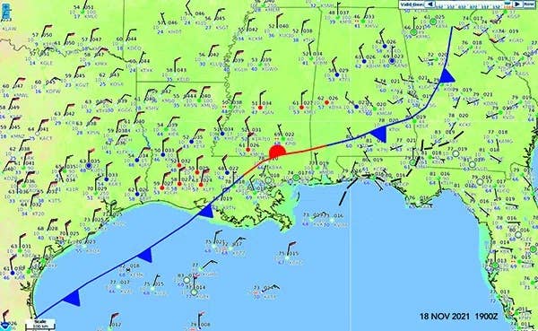
Such a map is shown below. You probably won’t want to import a map into drawing software like I’ve done, but it’s easy enough to eyeball the location of important boundaries. You’ll notice in my analysis, I didn’t simply assume all the areas of north winds mark a cold air mass, like those in the Gulf. Only when we go to the marked front location do we see temperatures fall poleward of the boundary.

That brings us to another important concept: Fronts are always on the warm side of a temperature transition zone; never on the cold side. Think about it—when a cold front is blowing through your location, has the front passed when temperatures begin to fall, or when temperatures have finished falling? The front passes when temperatures begin to drop, and that means the front passes first, followed by the thermal transition zone. This is closely reflected by what I’ve drawn on the map, with the temperature transitions found across Texas, Louisiana, Mississippi, and central Alabama.
Fronts Out West
The techniques described work well enough east of the Rockies, but it’s a different ball of wax out west. Terrain interactions, barrier flow, and unequal heating between valleys, ridges, and slopes predominate and overwhelm the temperature field, masking the true locations of fronts. The diurnal rise and fall of temperatures complicates things further. Even experienced aviation forecasters and meteorologists have trouble. What is a pilot supposed to do to keep tabs on the fronts?
Here it’s even more important to go to the Weather Prediction Center maps and look at not only the surface analysis but also the forecasts, so you can see where the fronts are and where they’re going. Again, these may require some refinement, but at least you have a heads up on what might be in the area.
It’s important to select some stations of interest and look at METAR trends over time. On Aviation Weather Center’s website under the METAR tab, there’s a station search box under “Request METAR data.” Set the dropdown tab for “Time” to “Past 36 hours.” I strongly suggest sticking with raw rather than decoded METARs, as changes will be easier to spot. This will give you all the observations from newest to oldest.

Using this METAR trend page, I find that wind direction and pressure changes provide some of the most important information. In the example for Boise, above, the wind direction provides firm evidence that a Pacific front has passed through the area. This is further confirmed by a rise in the altimeter setting. Although we are using secondary characteristics to find the front, none of the information disagrees with the temperature fall that we see at 0553 UTC. Though we do expect a temperature fall at that time, since 0553 UTC is at 11 pm Mountain Time and nighttime cooling is underway, we have a more abrupt temperature fall that confirms the passage of a front.
Notice that we also see gusty winds in the wake of the front. This is common in the postfrontal air, where the lowest few kilometers of the troposphere are destabilized due to fresh cold air flowing over a warm surface. In the eastern United States, this gusty wind behind the front is often accompanied by improvement in the ceilings and visibility, as dry air gets ducted to the surface. That’s not always the case west of the Rockies, though.
Fronts there often take on an “anafront” structure, where most of the dynamic lift is concentrated behind the front. This can produce precipitation trailing the front by up to 200 miles in its wake. The good news is most of the low ceilings will be in the form of scud clouds and obscuration from precipitation, rather than from fog and overcast stratus. If the TAF is above minimums behind a cold front, it’s likely the odds will remain in your favor.
Frontal Characteristics

Fronts can be classified into several types. First is the cold front—a front in which cold air, or greater density, is replacing the existing air mass. The warm front is the opposite; density will be lower as the front passes, implying the arrival of warm air. Structurally these two air fronts are similar except that a warm front has greater slope. In other words, the cold air is shallower at a given distance from the front. And with a warm front, there tends to be flow up and over the cold air, whereas with the cold front it’s the opposite. The anafront is the exception; there’s some flow up and over the cold front, leading to Pacific Northwest fronts having warm front characteristics even as they advance eastward bringing cold air at the surface.
Then there’s the stationary front. You’re probably aware of this as the “bad weather front.” There’s nothing special about the stationary front, and no unusual dynamic weather processes are occurring here. Rather it marks a line where neither air mass is replacing the other, prolonging the duration of any bad weather into hours and even days. A stationary front occurs in a few key situations: where density contrasts are weak, leading to weak pressure gradients; when terrain is blocking the progression of air masses, like we might find in the western Carolinas in winter; or where upper level winds oppose the low-level flow, leading to indeterminate flow.
Finally there’s the occluded front. This is simply a cold front that has caught up to a warm front, displacing the warm air aloft. This often complicates developing winter situations, where liquid precipitation is being formed aloft or melting is occurring, while subfreezing air is at the surface. If that’s the case, expect mixed precipitation forms along occluded fronts: rain, sleet, freezing rain, and snow, depending on what the air temperatures and wet bulb temperatures in the vertical column are like.
A special kind of front deserves mention: the outflow boundary. This is effectively a miniature cold front driven by a thunderstorm cold pool. It usually measures two to 20 miles in size and lasts a few hours, but can join with other outflow boundaries to produce a larger boundary measuring hundreds of miles long and lasting days. The only way to identify an outflow boundary is to look for the parent thunderstorm. This may require looking at radar charts earlier in the day. These larger outflow boundaries may at times behave like fronts, especially in the central United States in late summer, producing new areas of storms from day to day. The forecast models are not very good at predicting them beyond several hours, so it’s important to recognize when you’re looking at them and be aware the TAFs ahead of them may not be as accurate as expected.
There’s also the sea breeze, which is also like a miniature cold front. However instead of a cold air mass, we find a marine layer that moves inland from an ocean or lake. It’s most active during the morning hours, then weakens through the afternoon and becomes diffuse. If you’re near a coastal area, like Tampa or Los Angeles, it’s important to learn about sea breezes and look at some local hourly weather charts to watch how they behave. Though the models don’t handle these very well either, NWS aviation forecasters know to watch for these features in their forecast area and understand how to anticipate their behavior. As a result the TAFs you see that involve sea breezes should be fairly reliable.
Forecasters sometimes classify fronts further according to strength (weak, moderate, or strong), defined by the density contrast and the change over time. Strengthening of a front is called frontogenesis, which is favored in a convergent wind field, while weakening of a front is known as frontolysis and occurs in divergent flow. Up until the 2000s, you could find a three-digit code on the U.S. surface analysis that gives you all this information for each front. Regrettably, the trend toward computer modeling did away with this useful data.
Hopefully, I’ve been able to shed some light on the sometimes puzzling topic of fronts. The material I just discussed is part of the bedrock upon which forecasts are built. It’s likely there will be some morsel here that will help you unexpectedly in a difficult weather situation.
For more great content like this, subscribe to IFR!