


There’s no phenomena that shapes the flying experience quite like wind. It’s almost always present in some form. A crosswind makes for tricky landings, a gusty wind brings a bumpy flight, and a strong tailwind buys you an extra 15 minutes at your destination. It makes sense that this temperamental, fickle element should get an entire article of its own in hopes we can understand it a little better.
Where Wind Comes From
While pilots commonly think of wind as a chaotic entity that originates from various weather systems, forecasters recognize the unequal heating of the earth by the sun as the primary source of wind. This heating focuses mainly on tropical latitudes, setting into motion a convective-driven cell, the Hadley Cell, which rises in the tropical belt and flows poleward in the upper troposphere. There’s also a return branch in the lower troposphere that flows inward from the mid-latitudes. We recognize this return branch as the trade winds, a staple of weather in the Caribbean and in Hawaii. So immediately we can conclude that the trade winds are part of the Hadley Cell.
Mid-latitude weather is a little more complicated. It’s normally not powered by kinetic energy in the Hadley Cell, like the trade winds, but involves baroclinic weather systems, that is, weather systems created and maintained by sharp contrasts between hot and cold air masses. Some of the warm air is supplied by the Hadley Cell, but baroclinic systems create their own winds, including the jet stream. The systems that result are also self-supporting.
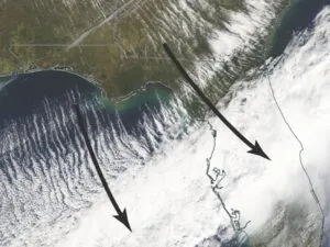
There are also what we call tertiary circulations. These are localized winds that develop due to uneven heating of mountains, lakes, and sea-land interfaces. Nowadays these types of winds are considered part of the domain of mesoscale meteorology, as they have scales of tens or hundreds of miles or less, and a life cycle measured in minutes or hours. This means that transient phenomena like thunderstorm outflow, hurricanes, and low-level jets are also part of this spectrum.
Most of the unexpected surprises at your destination, when the TAF busts, are due to the involvement of these mesoscale circulations. Today’s numerical models do a marginal job handling these features, and just 30 years ago they weren’t handled at all.
They form a sort of wildcard in the forecast, which means your weather briefings and TAFs are at a greater risk of becoming inaccurate when these phenomena are occurring. Situational awareness, an understanding of meteorology fundamentals, and getting up-to-date information will help you make sense of things when the weather gets confusing.
METAR Observations
Quite often the wind information you deal with comes straight from the ASOS or ATIS broadcast. This in turn comes from the METAR observation. Let’s take a look at it in more detail.
The first element we receive is the wind direction, given in degrees from where the wind is blowing, rounded to the nearest ten degrees. This can be referenced to either true north or magnetic north. A rule of thumb is national or “longline” dissemination, such as the official METAR report, encodes this value as true north. Local dissemination like you might hear on ATIS or from the control tower on final approach uses magnetic north.
Then there’s wind speed. A wind speed value by itself represents a “sustained” or “average” wind speed over a two-minute period at observation time. The units in most of the world are knots, equivalent to 1.15 mph, but in China, Russia, and North Korea you’ll get meters per second. Just double the value to get an approximate value in knots, or multiply by 1.94.
If there are 10 knots or more between peaks and lulls, a gust speed will be reported, and “G” will be encoded in the wind group of the METAR report. I find the presence of gusts to be incredibly useful for identifying areas of unstable air near the surface. Typically when I see gusts on the weather chart one of three things are happening: intense solar heating, a very cold air mass being modified as it passes over warm ground, or destabilization of the air mass as a whole as a strong weather system approaches.
Gusty winds are caused by increased vertical motion of the wind, and development of eddies, turbulent flow, and other “churning” motion. The same conditions that produce gusty winds also cause turbulence, so I tend to see them as part of the same spectrum of weather. That doesn’t mean gusty surface winds are associated with clear air turbulence (CAT) at 30,000 feet, but those gusty winds will at least produce mechanical low-level turbulence. If destabilization is happening aloft, clear air turbulence is also a possibility.
Backing And Veering
Backing and veering are adjectives that pop up a lot when we talk about the wind. They describe a change in wind direction. Veering always describes a clockwise change, such as from south to west, or north to east. Backing, on the other hand, is a counterclockwise change.
These terms are most often used to describe a change with respect to time. For example, if the TAF shows winds at 06Z are 13014KT, changing to 07020KT at 09Z, this indicates winds are backing with time.
We can also use the dimension of space. If the prevailing flow is southerly, “backed flow in the low levels” suggests a layer of easterly winds are present near the surface. “Backed flow north of the warm front” indicates winds are easterly north of that front. And “backing with height” means that the winds are becoming more easterly with height, given that same southerly prevailing flow.
Most of the time you’ll see this kind of usage in convective outlooks and other technical weather discussions. Tornadic storms strongly favor winds that are backed in the lowest kilometer of the troposphere (veering with height in that layer), so many high-risk storm days focus heavily on how this ingredient will shape the forecast.
One tidbit of interest: veering and backing are tied to a concept known as the thermal wind. We won’t get much into that, but suffice it to say that veering with height within a layer indicates warm air advection is present in that layer, that is, warmer air is replacing the existing air. The opposite, backing, indicates that cold air advection is taking place.
You can kind of combine these concepts together: a backing layer atop a neutral or veering layer means a trend towards “cold over warm”, which is the very definition of destabilization. This in turn suggests worsening weather is possible.
Pressure Gradient
So why does the wind blow? Wind is caused by the pressure gradient, the difference in pressure between two points. A vacuum cleaner is a great example; the motor creates a pressure deficit in the body, and air from outside rushes into the hose to fill the void, hopefully bringing some dust and crumbs with it.
You might point out that the vertical pressure gradient is a much stronger force. That’s absolutely correct. Just 25 miles above the surface, the pressure drops to one percent of that at sea level. The tendency of air to rush upward into space is opposed by the weight of the air itself. As a result, the air is in hydrostatic equilibrium and doesn’t move vertically except in convective currents, and in and around weather systems and terrain.
In the horizontal, pressure differences are referred to simply as the pressure gradient. A popular rule of thumb for assessing the pressure gradient is to look at the isobars on a weather map. Where they are close together, the pressure gradient is high, and winds will be fast-moving. From a forecasting standpoint, I’m far more interested in how these gradients vary from region to region than I am with the actual values of pressure. The gradients can also help find fronts, small-scale disturbances, and other interesting weather.
Another force exists because of the fact the Earth is a rotating body. Angular velocity from the earth’s rotation varies depending on the latitude, ranging from 0 mph at the poles to over 1040 mph at the equator. (Hold on to your hat!) This variation produces an apparent force that acts on any mass moving through the atmosphere, pulling it to the right (left in the southern hemisphere). The amount of force is directly proportional to the mass’s velocity.
We call this the Coriolis effect, or the Coriolis force. It acts in an opposite direction to that of the pressure gradient force. It’s not important in small-scale circulations like dust devils, tornadoes, or thunderstorm outflow, because Coriolis force is completely overwhelmed by other forces. For that reason, if anyone ever tries to convince you that the spin of water in a toilet bowl is influenced by the Coriolis force, just smile and change the subject.
But for air masses, jet streams, upper-level winds, and other atmospheric motion that evolves over hours and days, Coriolis force is very important. The Coriolis force and pressure gradient force balance each other, resulting in wind that’s in geostrophic balance. When this balance is upset, we get large areas of vertical motion that produce clouds and precipitation, and the TAFs start expanding ominously in size. The opposite of geostrophic balance is ageostrophic flow, and it’s often caused by a quasi-geostrophic disturbance or QGD. Much of a forecaster’s work revolves around finding these QGDs and trying to figure out how they will shape the weather.
Coriolis force is zero at the equator, is weak in the tropics, and is very strong at high latitudes. This has some interesting effects with systems like hurricanes. If you’ve ever wondered why tropical cyclones don’t strike places like Singapore, Venezuela, and Indonesia, it’s because they’re near the Equator. The lack of Coriolis force allows wind to flow directly into any low pressure area and to fill it rapidly. Tropical cyclones simply can’t develop the pressure falls that are needed to get themselves underway.
An opposite effect is found at the poles. The pressure gradients you see on weather charts don’t produce as much wind in polar regions as you might expect. The Coriolis force is strong at these latitudes, and by opposing the flow of air into low pressure areas, it reduces the kinetic energy of the wind. That’s not to say Bering Sea and Icelandic lows and the wind they produce won’t get intense, but winds of over 100 mph are not very common.
The final force that’s important is frictional force. This is caused by drag as winds move over mountain ranges, rough terrain, forests, oceans, and buildings. It acts opposite to the forward motion of the air. One interesting effect of friction is by slowing the wind down, it reduces the Coriolis force.
Remember, Coriolis force is proportional to velocity. The pressure gradient remains the same, so the winds change direction and move more directly into low pressure areas and out of high pressure regions. In the middle and upper troposphere, and over oceans, friction is negligible and the wind closely follows the isobar field, crossing it only at modest angles.
Upper-Level Winds
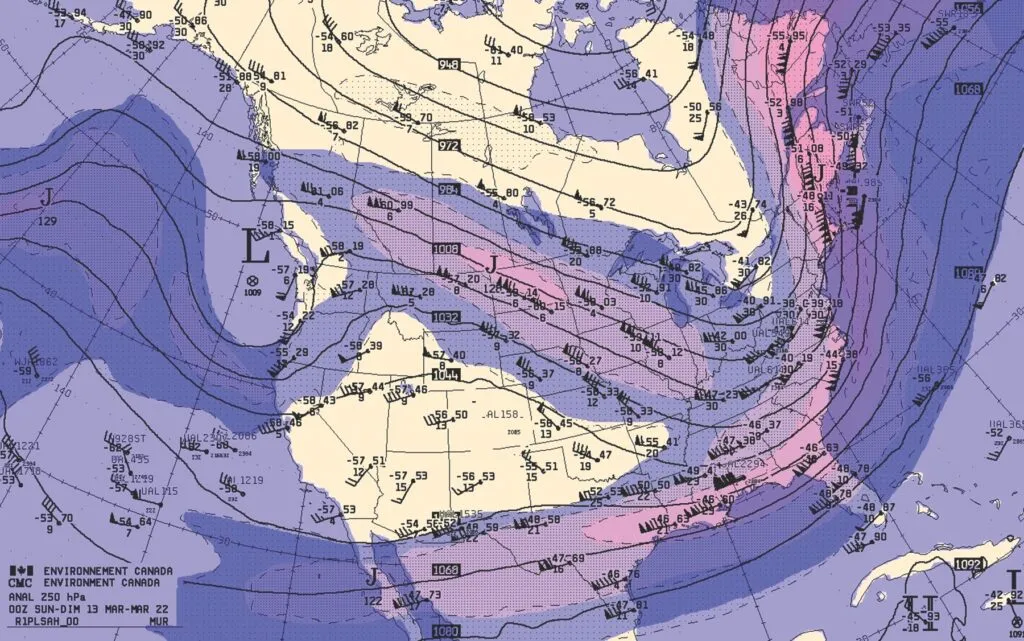
If surface winds are shaped by surface highs and surface lows, why do upper-level winds exist? You’re likely well acquainted with the polar jet stream. This is a band of strong winds ringing each hemisphere that closely follows the polar front. The polar jet is directly caused by the temperature gradients in the lower troposphere, the same ones that define the surface fronts.
Without getting into the technical details of upper-level winds, I’ll give you a few useful rules of thumb. The most important rule for upper-level winds is when your back is to the wind in the Northern Hemisphere, the surface cold air mass will be found on your left, and warm air on your right. This concept can help you visualize the weather as you fly along on a cross-country route.
Upper-level wind shear is closely correlated to CAT. This is especially true with vertical shear. In the golden era of jet travel, when Boeing 707s and DC-8s roamed the skies, airline forecasters worked almost entirely from hand-computed shear values to forecast CAT. Thankfully today we now have sophisticated Graphical Turbulence Guidance charts to look at, in addition to trustworthy SIGMETs, but occasionally when looking at weather charts you might see strong layers of shear and you’ll know to tighten your seatbelt.
And finally for those with a wind readout on their multifunction display: a decrease in wind speed with height at jet stream level is a good indicator that you’re transitioning into the stratosphere. The jet stream core is almost always located in the very top layers of the troposphere. In the stratosphere, the high wind velocities found above the polar fronts diminish, and the small-scale eddies that cause clear air turbulence are suppressed.
This article originally appeared in the June 2022 issue of IFR magazine.
For more great content like this, subscribe to IFR!

One wind prediction that I find is usually very inaccurate is winds aloft at low levels. For example, returning from Sun N Fun Sunday to Virginia my 430W measured the winds at 7,500ft to be from the east whereas the forecast was for them to be from the west. Velocity was pretty close, however. Is the GPS wrong?
“There’s no phenomena that shapes the flying experience…”
That’s “There’s no phenomenon…” Singular.