A Radar Primer

Radar, whether we’re talking air traffic control, thunderstorm detection, navigation, or even air combat, is a technology that has shaped the history of flight in countless ways. The word “radar” is an acronym (RAdio Detection And Ranging) and was coined in 1939 by the United States Army Signal Corps as it worked on these systems for the Navy. Its rapid development during World War II is still well known in the aviation community and it’s often associated with that era.

A Brief History

The science of radar goes back half a century earlier when the physicist Heinrich Hertz demonstrated the characteristic of electromagnetic waves to reflect off objects. In the earliest decades of the 20th century, it was suggested that electromagnetic reflection could be harnessed to detect ships in coastal areas and harbors, but there was little interest.

In the mid-1930s, the United States, England, Germany, and the Soviet Union simultaneously developed the first radars for aircraft detection. As World War II descended on Europe, this technology was quickly put to work by England for the Chain Home early warning radar network. The U.S. Army produced numerous SCR-270 radars, one of which detected the Pearl Harbor attack in 1941.

World War II jumpstarted a series of massive improvements in radar reliability, quality, and display technology. By the end of the war, the familiar circular radar scope, or plan position indicator (PPI) in which echoes were “painted” on the screen, became a standard part of the radar console. A series of refinements in the 1950s led to the modern WSR-57 radar, which served to 1996.

Two significant radar technology developments arrived in the 1970s. With the arrival of minicomputers, radars nationwide were retrofitted with Digital Video Integrator Processors (D-VIP) that converted radar data from analog to digital. Echoes could be displayed as colored pixels on a screen with a digital map and transmitted digitally over the telephone lines. The Weather Channel often used these Kavouras dial-up images on their “radar stops” in the 1980s. Airline pilots from that era viewed these radar pictures in their dispatch offices.

The second significant development was Doppler radar. Early studies in 1958 showed that velocity measurements were extremely effective at finding tornadoes. This led to a substantial amount of development work in the late 1970s and early 1980s by the National Center for Atmospheric Research and the National Severe Storms Laboratory. Retrofitting the old radars was not practical, and it was clear a new purpose-built radar was urgently needed, one based on modern computer technology. This new radar program was called NEXRAD (Next-Generation radar) and was referred to as the WSR- 88D. The specifications were locked down in 1988, and the first radars were commissioned in 1992. Overall, 160 radars were installed between 1992 and 1999.

Wavelength And Weather

Radar works in two steps: transmitting a directional electromagnetic pulse, then listening for the reflected signal. A radar pulse moves at the speed of light, about 300,000 kilometers per second. So, if it takes a pulse one millisecond to return, you know that the total trip distance is (300,000 × 0.001) 300 kilometers meaning the target is 150 kilometers away.

The pulse is tuned to a specific radio frequency, given in MHz (millions of waves per second) or GHz (billions). This frequency is fundamental because it shapes what we can do with the radar signal. Since the speed of light is a constant, each frequency also corresponds to a specific wavelength.

As an example, transmit a pulse of 300 MHz for one second. This wavetrain will move 300,000 km (300 million meters), and since we’re transmitting at 300 MHz, it will be composed of 300 million waves, each with a length of one meter. In another example: three GHz is 10 times the frequency and produces 10 times as many waves, so we get a wavelength of 0.1 m (10 cm).

This is the operating frequency for NEXRAD and why it’s classified as a “10-centimeter radar.” We also refer to this as the S-band—an IEEE radio band that stands for “short wavelength.”

Wavelength is essential because if the size of the waves is much bigger than the size of the material that makes up the target, little energy will be reflected, and it will be harder to detect the signal. As you might guess, an S-band radar produces waves that are much bigger than most weather phenomena, and it’s not very sensitive to drizzle, and it rarely detects clouds. S-band radars are also costly, requiring a large antenna, and require more power. However, these wavelengths deliver a powerful punch through dense precipitation. In other words, they have low attenuation.

If you have airborne radar in your cockpit, chances are it transmits pulses in the X-band. This band was named after the shape of crosshairs because state-of-the-art Eagle fire control radars carried aboard B-29 bombers were X-band radars. The X-band is centered near 10 GHz that yields a wavelength of about three cm. This is much shorter than the S-band. Since this wavelength more closely matches precipitation, it will more readily detect smaller droplets. But these shorter wavelengths are more highly attenuated, and as a result, the weather displayed beyond heavy precipitation will often look weaker than it really is.

In between the S-band and X-band is the C-band centered on six GHz (five cm). The letter C was chosen for “compromise.” This provides some of both worlds, allowing acceptable performance in heavy rain with good sensitivity and low cost. An excellent example of a C-band radar is TDWR (Terminal Doppler Weather radar), a five cm radar. Another example is the WSR-74, a low-cost National Weather Service (NWS) radar that was used up until the 1990s.

Products

The primary radar product you’re familiar with is reflectivity showing where weather echoes are and their intensities. These only show precipitation. Operational weather radars do not normally detect clouds. There are some exceptions, primarily when NEXRAD is operating in “clear air mode,” which is more sensitive. But you will not see cumulonimbus clouds represented on radar. Instead you’ll just see their precipitation field.

A second key radar product is velocity. You don’t deal with this in the cockpit, but forecasters are interested in velocity products as they show not only the clear air wind field but the flow within thunderstorms.

The third radar product is spectrum width—a measure of the diversity of velocity that it detects at each point. Forecasters ignored spectrum width for over a decade, but in recent years it has begun attracting attention for its value in revealing boundaries, tornado debris clouds, and other fine-scale structures. High spectrum width values are displayed as a “turbulence” marking on many airborne radars; that’s valuable since it’s a direct measurement.

Scan Strategy

You’ve likely noticed the ATC radar antennas at airports and how they spin around every few seconds. Weather radars work like this, but their antennas rotate slower to extract more data. Weather radar antennas are also highly directional, casting all their energy in a one-degree cone instead of a wide fan.

While ATC radars are tilted upward to observe as much of the sky as possible, the classic weather radar presentation is tilted just above the horizon, commonly at an elevation of 0.5 degrees. This is often referred to as the low-level scan.

The original NWS radars in service until the 1990s always operated at this elevation, except when the operator was manually controlling the antenna to measure storms. Nearly all NEXRAD images of severe storms, particularly those showing hook echoes, also use the low-level scan.

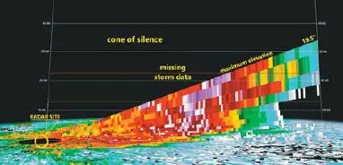
Since the 0.5-degree elevation beam starts at the ground and only reaches 10,000 feet when it gets 80 miles away, the radar beam will frequently undershoot weather, especially thunderstorm clouds—potentially missing a significant amount of information. So, the NEXRAD unit employs a scan strategy that starts with the low-level tilt and adds additional elevations, such as 1.5 degrees, 2.4 degrees, 3.4 degrees, up to a maximum of 19.5 degrees. These are combined into a snapshot known as volume scan.

The individual scans take about 30 seconds, adding up to a volume scan that takes three to five minutes to complete before individual scans can be gathered again. Therefore, it can take many minutes to get new radar data from a NEXRAD site.

Varying the pulse repetition frequency gives pros and cons in terms of usable range and maximum unambiguous velocity. We can also vary the scan patterns and radar operating characteristics within a volume scan, depending on whether we want to get scans faster or get more accuracy. NEXRAD engineers have worked hard on this problem over the past 20 years and have devised several automatic scan strategies called volume coverage patterns (VCPs) that can be selected depending on the weather.

The VCP number at any moment is usually given in the legend, and you can look up the information to see exactly what it means and how fast the products will come out. A couple of VCPs are designed to provide “clear air mode,” in which the antenna rotates slowly and sensitivity is increased. A clear air volume scan takes 10 minutes, but it accurately detects the wind field and often picks up cloud layers. If the radar data looks a little weird and the weather is VFR, the radar is probably just operating in clear air mode.

You might have found it surprising that the maximum NEXRAD antenna tilt is 19.5 degrees. Look out your window, stretch out your arm, put your thumb tip on the horizon, and spread your pinky upward. The arc covered by your hand is about the same volume as a NEXRAD volume scan. Everything above your pinky would be missed by the radar. That’s a huge chunk of the sky. Forecasters refer to this as the cone of silence. The radar never knows what’s happening there.

Another problem is that the antenna is so low that ground clutter interferes with the display within a few miles of the radar site. These issues can make it hard to analyze a storm that’s close to a radar site. Neighboring radars can be used temporarily to analyze storms that are passing through this cone of silence.

BREF And CREF

Perhaps you wondered if it’s possible to combine all the different reflectivity scans into a master scan that uses data for all levels. This is a common product called composite reflectivity (CREF). This is different from base reflectivity (BREF) that uses a single scan, usually from 0.5 degrees.

Base reflectivity is used most often by forecasters as it unravels the small-scale structure near the ground and reveals hook echoes, bow echoes, boundaries, and other features. Composite reflectivity is best for pilots since it always presents the most intense echo at each point, either near the ground or 40,000 feet. But that’s also one of its downfalls, as the maps are a jumble of data at all levels. Useful patterns in a fast-breaking situation may be obscured. Also, composite reflectivity is not immune from missing data within the cone of silence. Radar mosaics are effective in filling in these gaps and should be used where possible.

Most aviation weather products like radar mosaics, especially those on SiriusXM, use a composite reflectivity display, so nothing is missed. Some radar products from other sources, like those on the web, use base reflectivity. Airborne radar should be thought of as a base reflectivity product since it doesn’t present a large volume of the storm at once.

When you start using a new radar source, it’s essential to understand which type of radar reflectivity is being observed. If it’s not provided in the legend or the product help, go to an Internet radar source like College of DuPage Weather, bring up the individual radar, and compare the BREF and CREF products to your sample image to see which one matches.

One Final Word

Although we haven’t talked about weather signatures, now you know where your data is coming from and have a better grasp on the terminology. This information can yield insight into why you might be seeing delayed information or unusual images. And perhaps now you understand the difference between base and composite reflectivity, which are quite different.

That said, the United States freely distributes its radar data, and you can get even the most obscure NEXRAD products on various websites. There’s only one way to get better at using a product—practice. So next time there’s a storm in your area, try pulling up various radar products to see what’s going on. Immerse yourself and build your skills.

Tim Vasquez has done most of his 30 years of forecasting on the Great Plains, and continues to program, write weather books, and process weather data from his home office in Texas.

This article originally appeared in IFR magazine.

For more great content like this, subscribe to IFR!